Excel isn’t a database, but that hasn’t stopped people from using it as one.
People have been doing this since early versions of Excel and creating relationships between different tables using VLOOKUP or INDEX and MATCH.
The good news is that more and more database-like functionality is being added with each version, and since Excel 2013 we’ve been able to add relationships to tables.

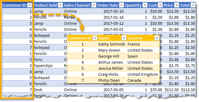
This example has an Orders table that contains data related to customer orders such as the Customer ID, Product Sold, and the Total.
Another table called Customers has the Name and Country for each Customer ID. But what do you do if you want to analyze the Orders data by customer Name or Country?
One solution would be to add two more columns to the Orders data and use a VLOOKUP function to bring in the customer Name and Country based on the Customer ID.
Another more elegant solution would be to use the pivot table Data Model to create a Relationship between the Orders table and the Customers table using the Customer ID field in both tables.

Create a table based on the Orders table.
Go to the Insert tab in the ribbon and select Pivot Table from the Tables section.
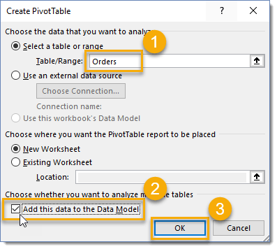
From the Create PivotTable menu.
Repeat these steps for the Customers table.
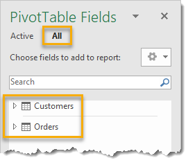
With either of your pivot tables created, you should see both tables in the PivotTable Fields window from the All view.
You can delete one of the pivot tables created since you only need one, the data will remain in the Data Model.
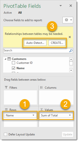
Build your pivot table with the Name from the Customers table in the Rows area and Total from the Orders table in the Values area.

If you choose Auto-Detect, Excel will work to create the relationships and you can check the results by pressing the Manage Relationships button or just Close the window.
With this simple relationship, Excel is easily able to create the relationship. Small tables and consistent field names between tables will help Auto-Detect to work.

If you choose to Create the relationships yourself then the Create Relationship menu will open.

Now your resulting pivot table contains the customer Name from the Customers table along with the correct corresponding Total from the Orders table.
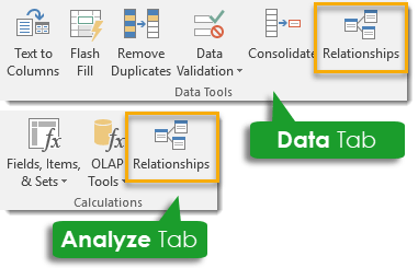
You can also create these relationships before trying to build the pivot table. You can do this from either the Data tab or the Analyze tab in the ribbon.
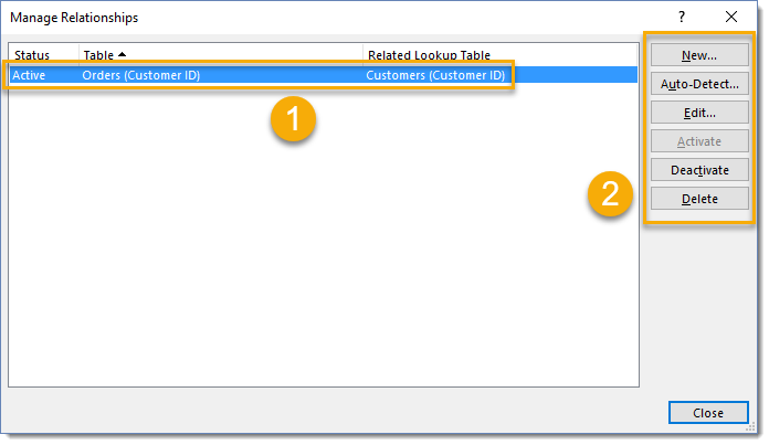
This will open the Manage Relationships dialog box.
This is an awesome way to avoid VLOOKUP or INDEX and MATCH, and minimize the columns in your tables.